Alohamora
Boundary Detection and Image Recognition
Phase 1
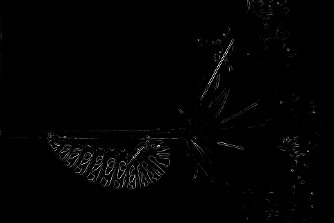
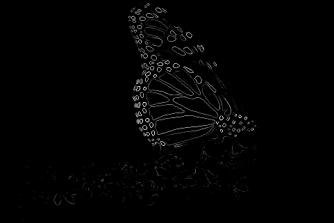
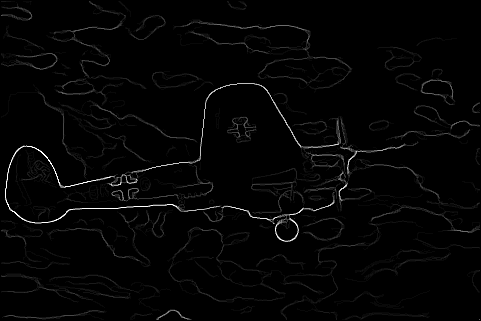
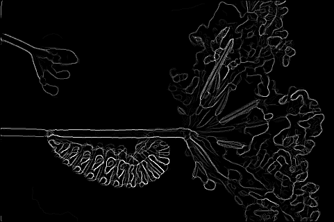
Implementation of Pb-lite boundary detection algorithm using filter masks with a comparison to baseline Canny and Sobel outputs.
Process Overivew
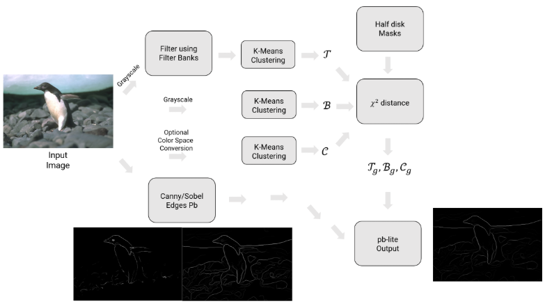
The pb (probability of boundary) boundary detection algorithm significantly outperforms classical methods by considering texture and color discontinuities in addition to intensity discontinuities. Qualitatively, much of this performance jump comes from the ability of the pb algorithm to suppress false positives that the classical methods produce in textured regions. In this home work, a simplified version of pb is developed, which finds boundaries by examining brightness, color, and texture information across multiple scales (different sizes of objects/image). The output of the algorithm is a per-pixel probability of being a boundary. The simplified boundary detector is evaluated against the well regarded Canny and Sobel edge detectors. A qualitative evaluation is carried out against human annotations (ground truth) from a subset of the Berkeley Segmentation Data Set 500 (BSDS500).
Filter Banks
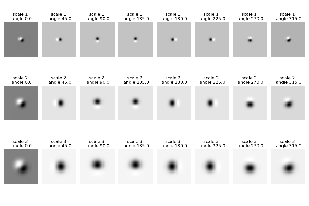
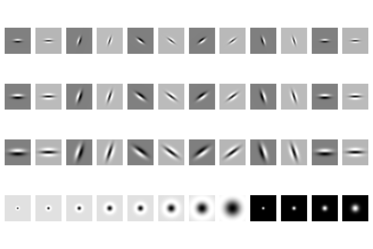
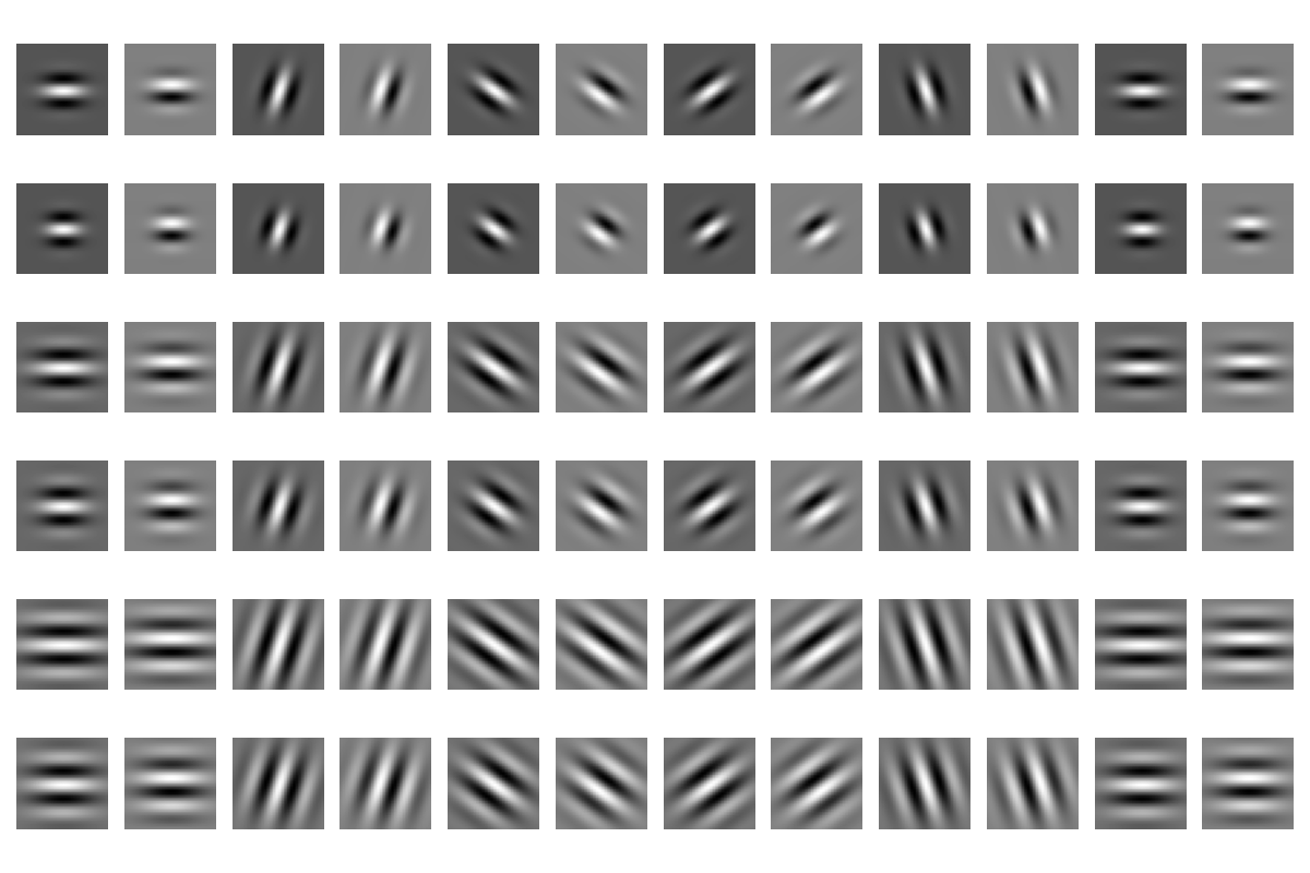
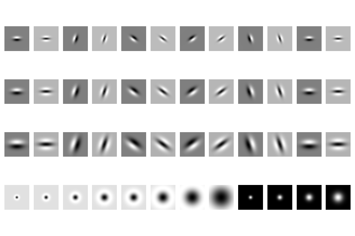
The first step of the pb-lite boundary detection pipeline is to filter the image with a set of filter banks. Three different sets of filter banks have been created for this purpose:
- Oriented Difference of Gaussian (DoG) Filters
- Leung-Malik (LM) Filters
- Gabor Filters
Texton Map
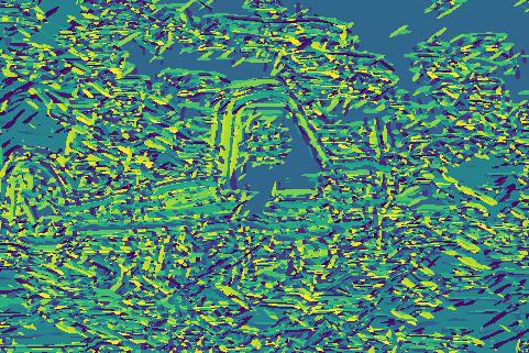
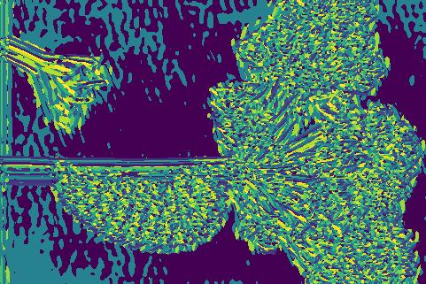
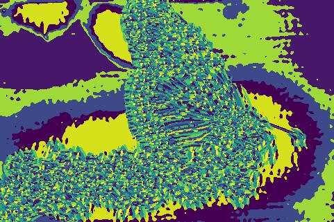
Filtering an input image with each element of the filter bank results in a vector of filter responses centered on each pixel. If the filter bank has N filters, then there are N filter responses at each pixel. A distribution of these N-dimensional filter responses could be thought of as encoding texture properties. This representation is simpyfied by replacing each N-dimensional vector with a discrete texton ID. This is done by clustering the filter responses at all pixels in the image in to K textons using kmeans clustering. Each pixel is then represented by a one-dimensional, discrete cluster ID instead of a vector of high-dimensional, real-valued filter responses known as “Vector Quantization”. This can be represented with a single channel image with values in the range of [1,2,3,…,K] where K=64.
Brightness Map
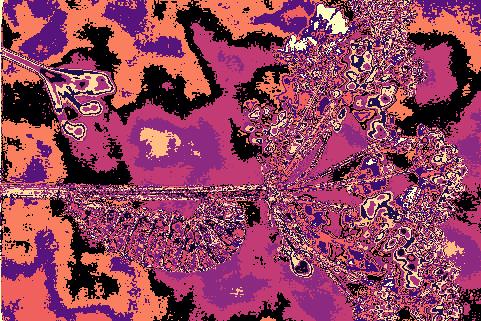
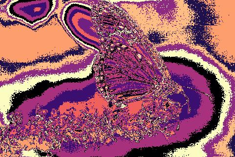
The concept of the brightness map is as simple as capturing the brightness changes in the image. Again the brightness values are clustered using kmeans clustering into 16 clusters.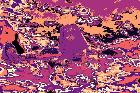
Color Map
The concept of the color map is to capture the color changes or chrominance content in the image. Again the color values are clustered using kmeans clustering into 16 clusters.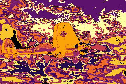
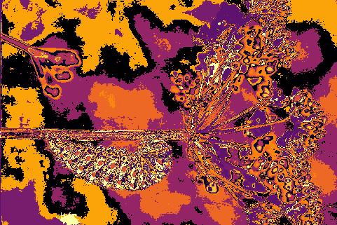
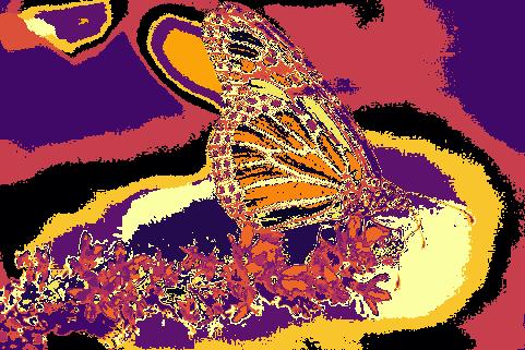
Texton, Brightness and Color gradients
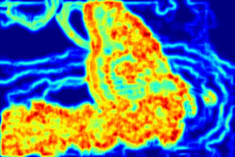
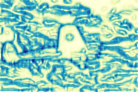
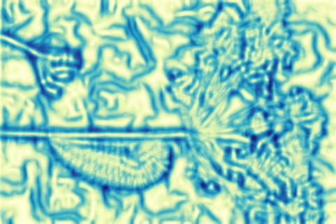
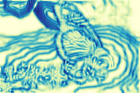
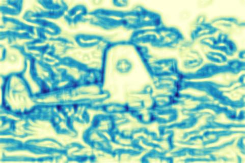
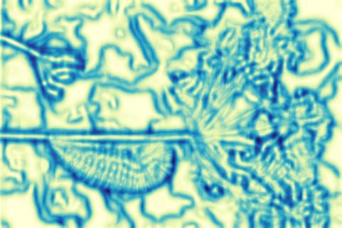
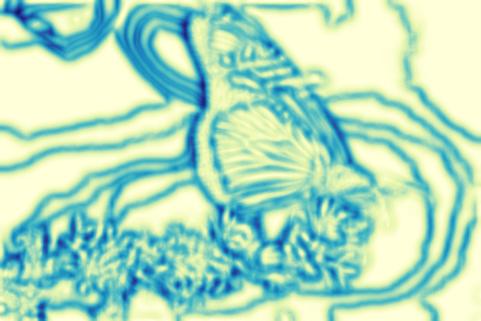
To obtain these gradients, we need to compute differences of values across different shapes and sizes. This can be achieved very efficiently by the use of Half-disc masks. The half-disc masks are simply pairs of binary images of half-discs. This is very important because it will allow us to compute the (chi-square) distances using a filtering operation, which is much faster than looping over each pixel neighborhood and aggregating counts for histograms. These gradients encode how much the texture, brightness and color distributions are changing at a pixel and are computed by comparing the distributions in left/right half-disc pairs. If the distributions are the similar, the gradient is small and if the distributions are dissimilar, then the gradient is large. Because the half-discs span multiple scales and orientations, a series of local gradient measurements are obtained encoding how quickly the texture or brightness distributions are changing at different scales and angles.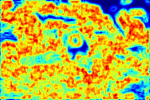
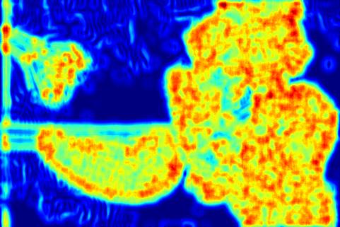
Boundary Detection
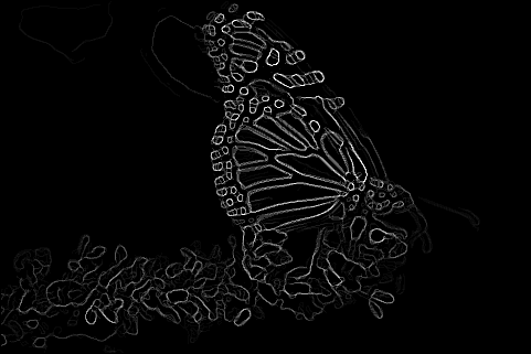
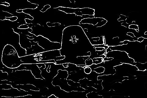
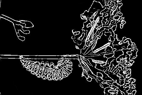
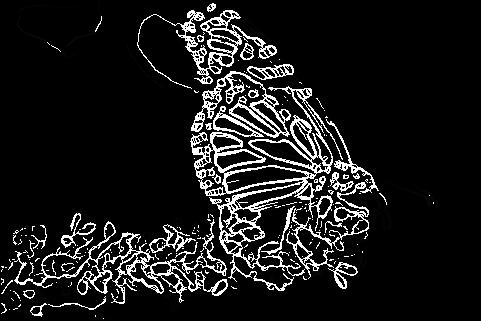
The pb-lite boundary detection algorithm is finally applied to the images. To calculate the final filtering kernel from the earlier kernels, the Tg , Bg and Cg averaged to create a single kernel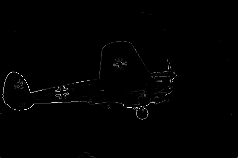
Phase 2
In this phase multiple neural network architectures are implemented and compared on various criterion like number of model parameters, train and test set accuracies.Process Overivew
The primary objective is image classification using Neural networks. The model is trained on the CIFAR-10 dataset. There are a total of 60000 images in the dataset which are split into 50000 train images and 10000 test images. There are 10 classes in the dataset and the output of the model is a probability of the 10 classes while the input to the model being a single image. The training is performed using the PyTorch library.Data Preprocessing
The training part:- The images are normalized between 0 and 1
- flipped horizontally
- rotated by a maximum of 30 degrees
- randomly affined
- jittered on color
Base Model
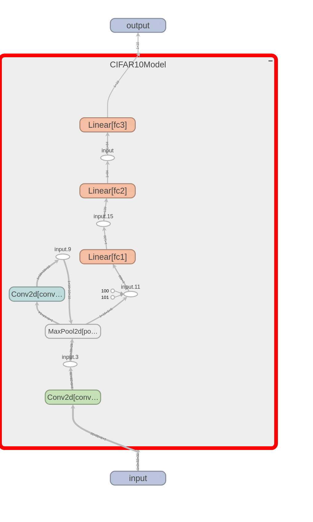
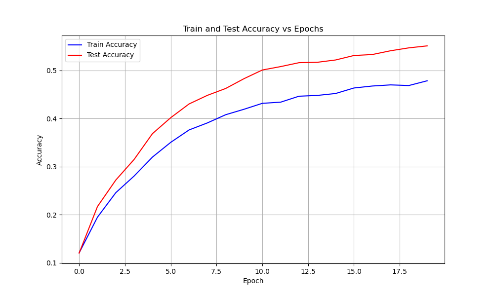
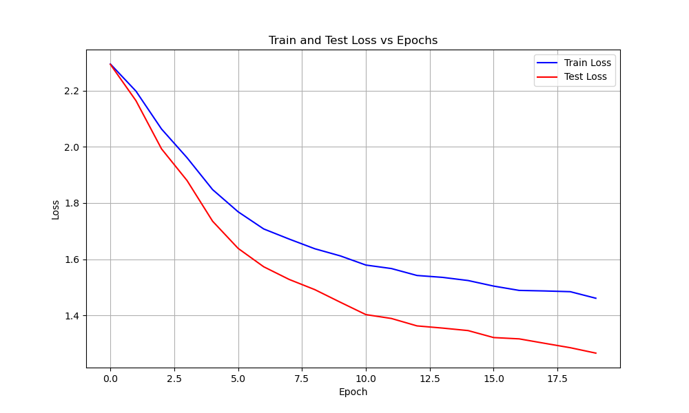
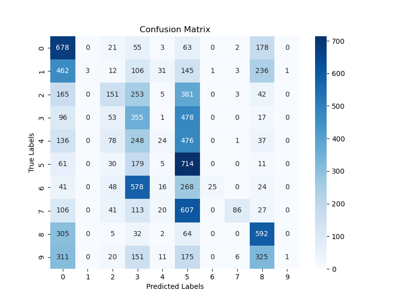
The Base Model is a basic convolutional network. Hyperparameters: The hyperparameters used to train the Base Model as are follows:- Learing rate: 0.01
- Batch size: 32 — 64 — 256 — 512

Normalized Model
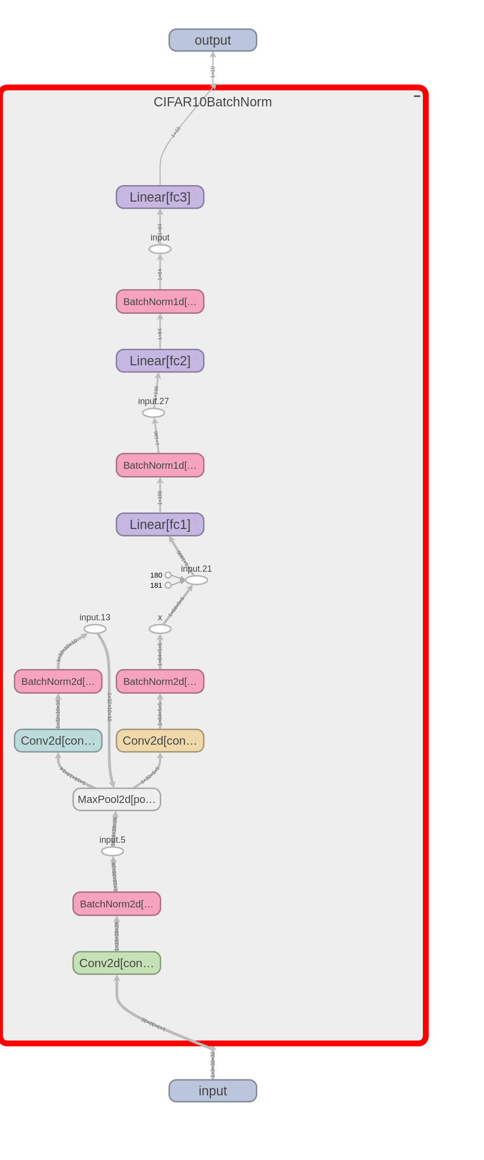
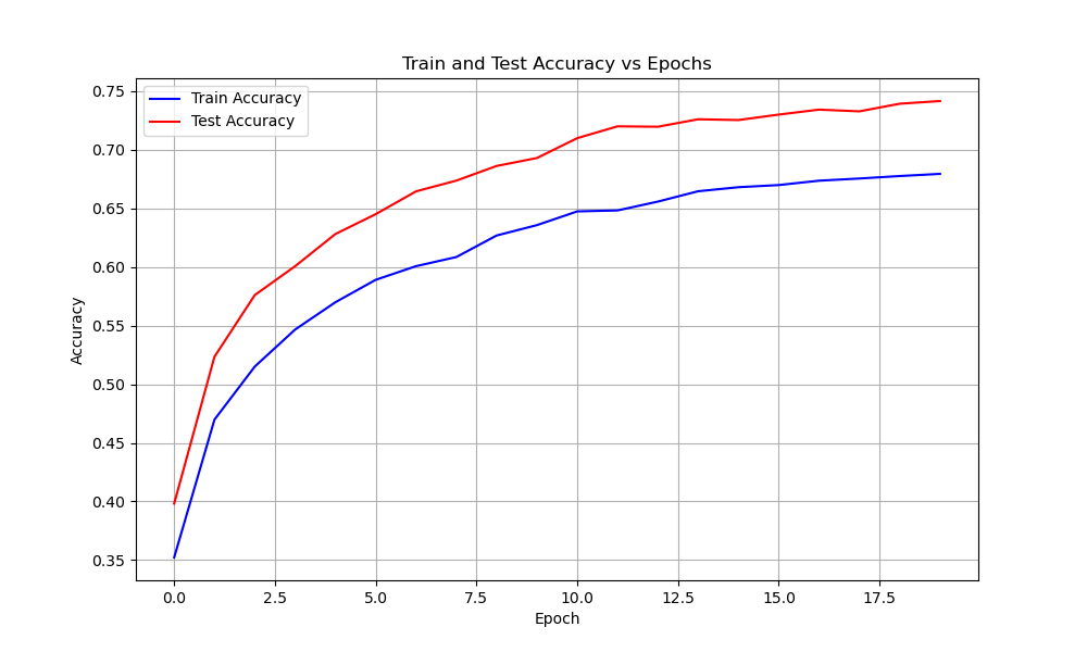
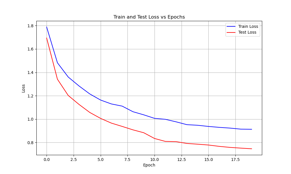
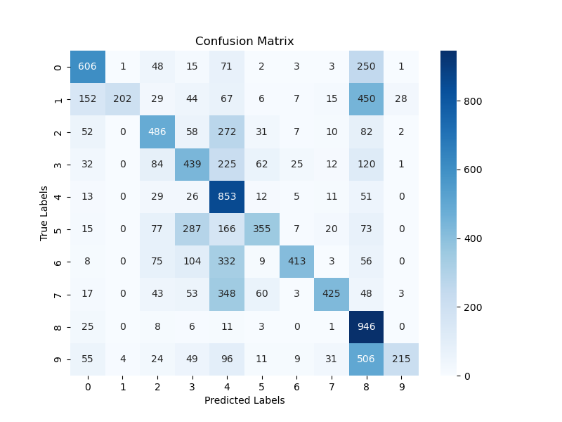
The Base Model is modified to include a batch normalization layer in between each convolutional layer. Hyperparameters: The hyperparameters used to train the Base Model as are follows:- Learing rate: 0.01
- Batch size: 64 — 256 — 512
- Number of epochs: 20 — 50 — 75
- Optimizer: SGD
- Activation: ReLU
- Loss Function: Cross Entropy

ResNet Model
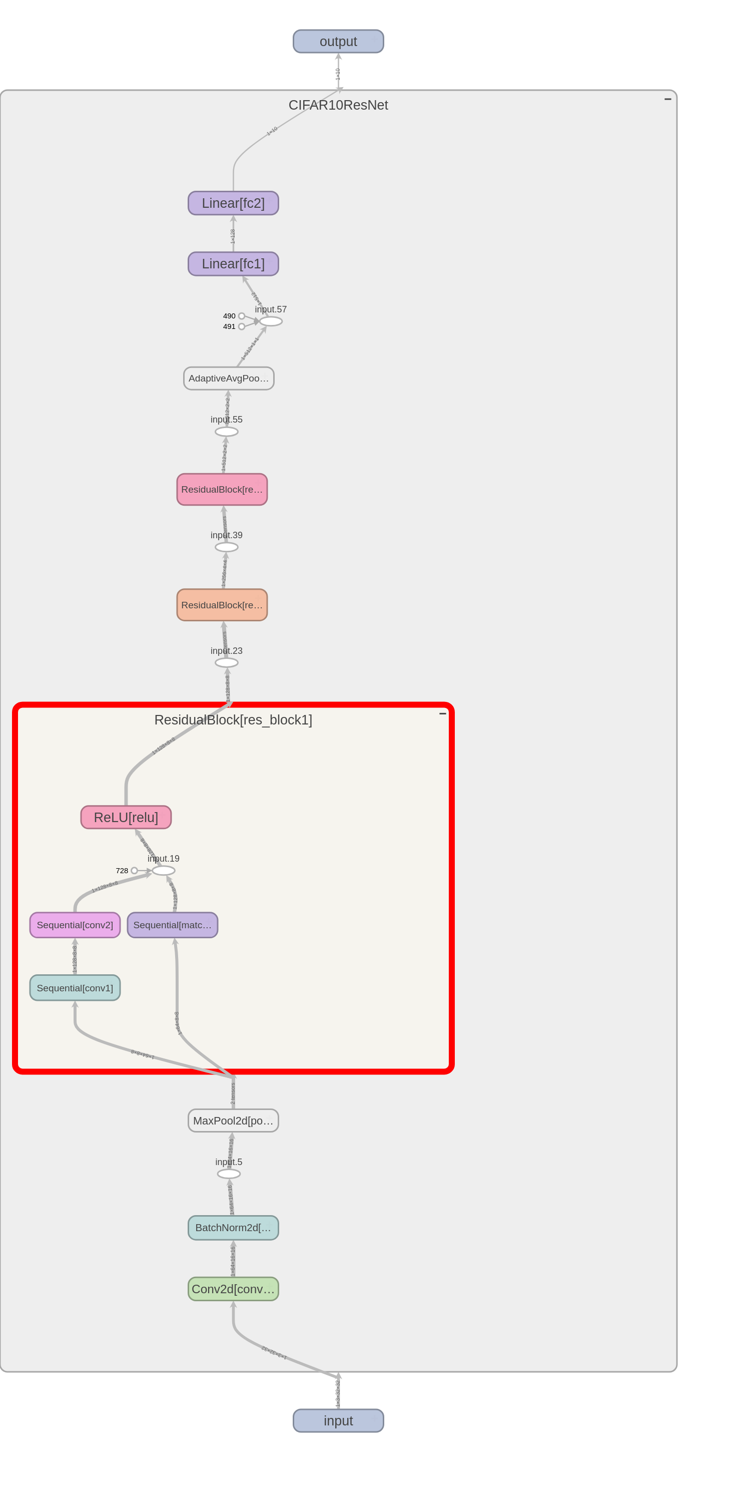
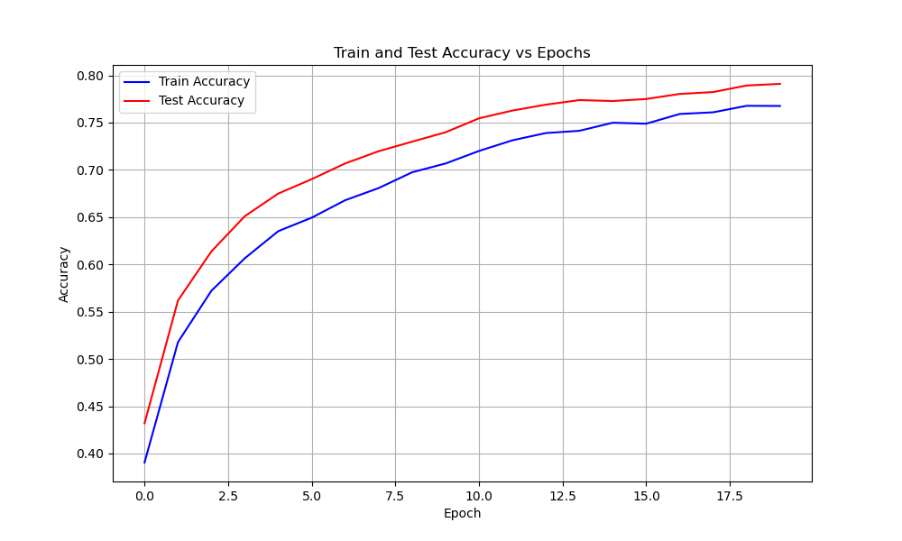
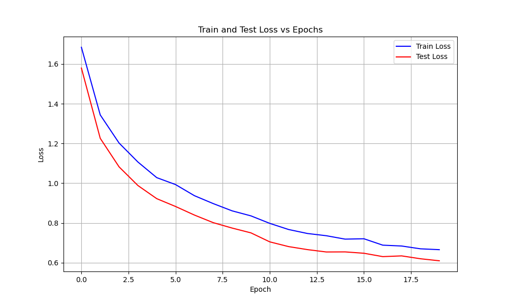
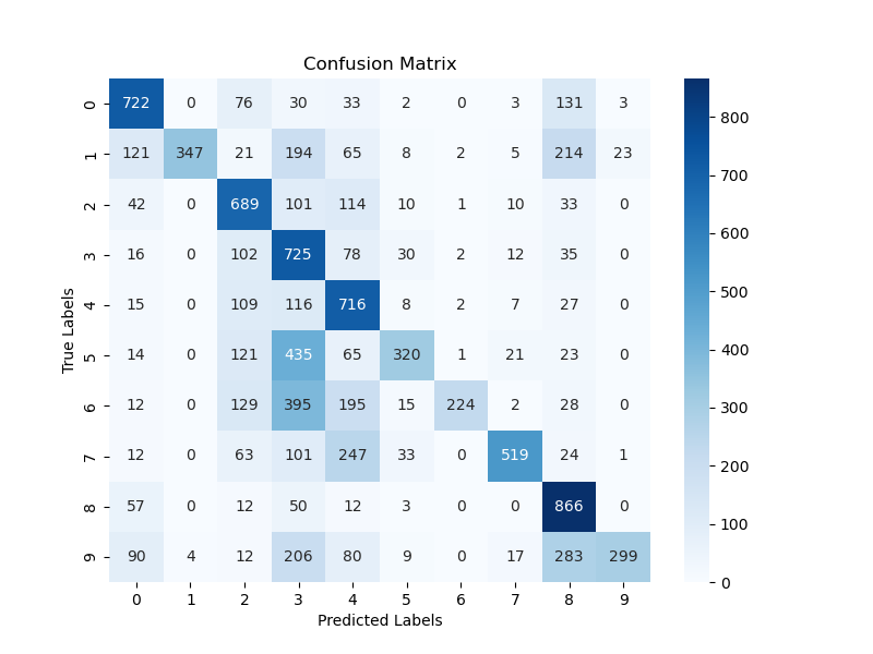
By adding shortcut connections to the Base Model a Residual Network or ResNet can be constructed. Deep networks often show behaviour of degradation in training accuracy due to saturation. Residual networks overcome this degradation by using shortcut connections. Hyperparameters: The hyperparameters used to train the Base Model as are follows:- Learing rate: 0.01
- Batch size: 64 — 256 — 512
- Number of epochs: 20 — 50 — 75
- Optimizer: SGD
- Activation: ReLU
- Loss Function: Cross Entropy

ResNeXt Model
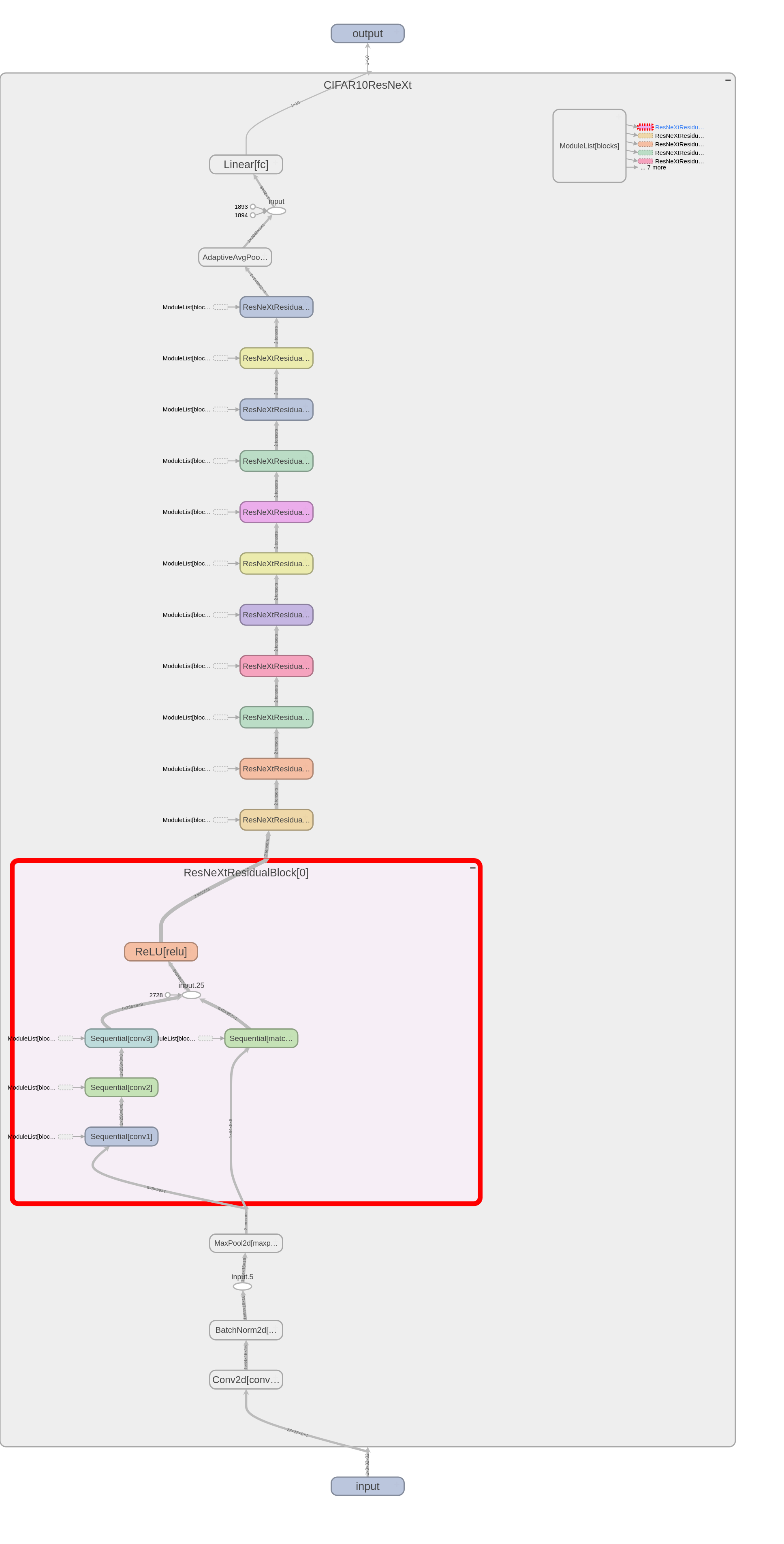
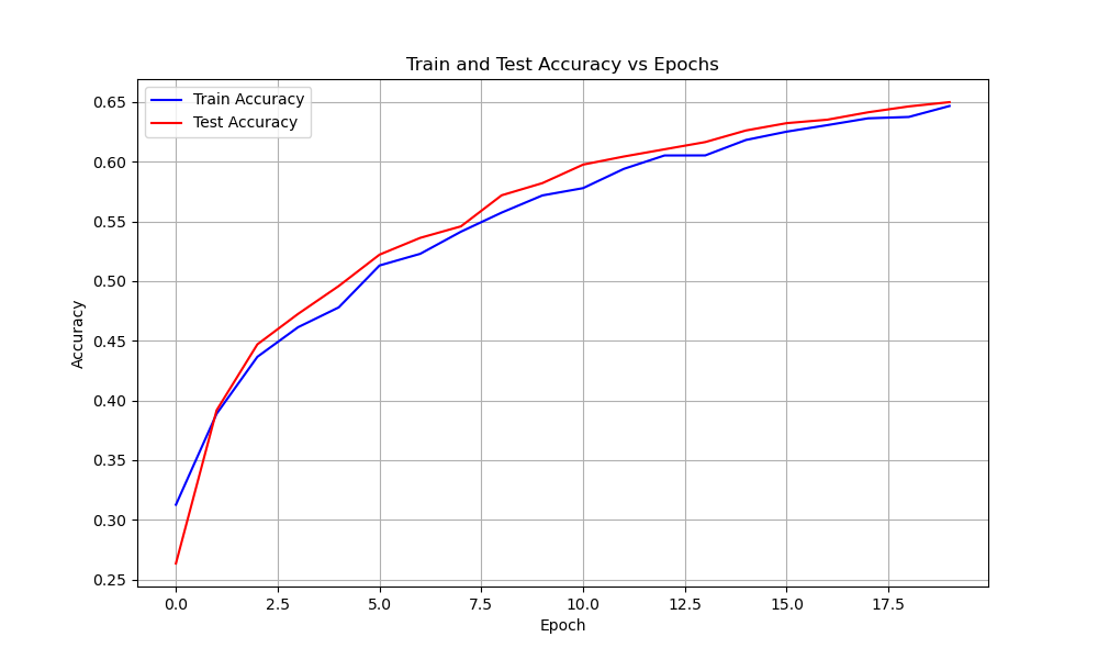
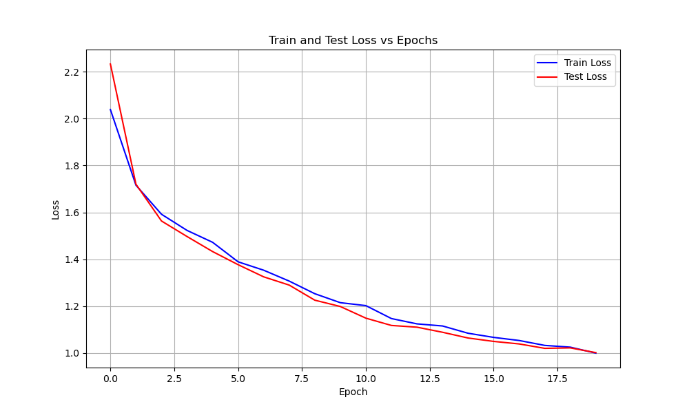
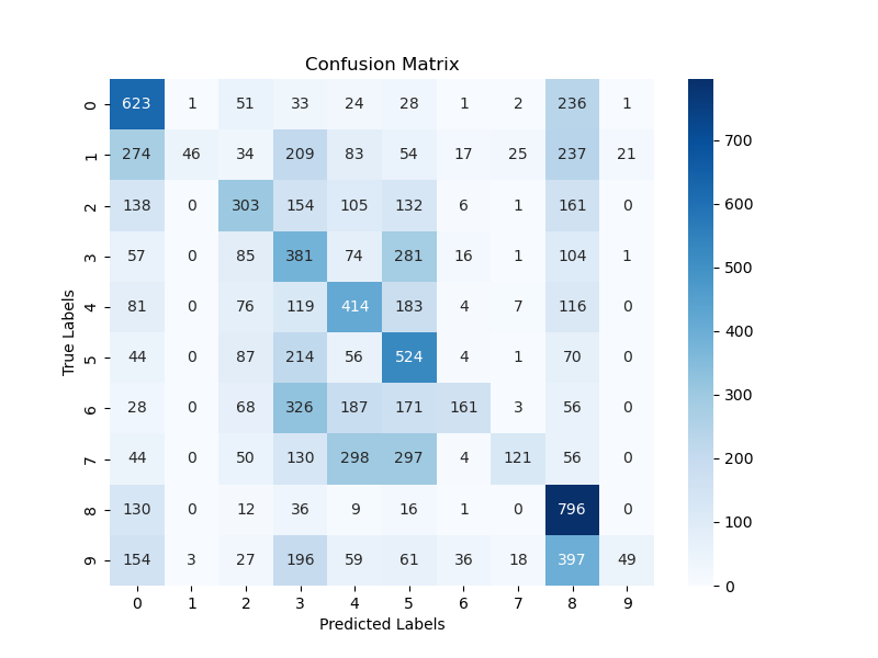
The ResNeXt models are highly modularized models which are constructed by repeating a building block that aggregates a set of transformations with the same topology. This results inn a simple, multibranch architecture requiring only a few parameters to be set. ResNeXt present a new dimension called as cardinality which is essentially nothing but the size of the set of transformations as an additional dimension to the existing dimensions of depth and width. Hyperparameters: The hyperparameters used to train the Base Model as are follows:- Cardinality: 32
- Learing rate: 0.01
- Batch size: 64 — 256 — 512
- Number of epochs: 20 — 50 — 75
- Optimizer: SGD
- Activation: ReLU
- Loss Function: Cross Entropy

DenseNet Model
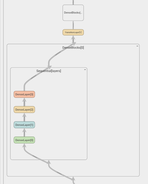
From ResNet it is safe to say that convolutional networks can be substantially deeper, more accurate and efficient to train if they have shortcut connections. While Base Model having L layers, has L connections, the Dense Convolutional Network has L(L+1)/2 connections in its network. For each layer, the feature maps from all the preceding layers are used as inputs, and its own feature maps are used as inputs in all subsequent layers. DenseNet models alleviate the vanishing gradient problem due to the shortcut connections. Hyperparameters: The hyperparameters used to train the Base Model as are follows:- Growth rate: 16
- Learing rate: 0.01
- Batch size: 64 — 256 — 512
- Number of epochs: 20 — 50 — 75
- Optimizer: SGD
- Activation: ReLU
- Loss Function: Cross Entropy

Model Comparisons
| Model | Accuracy Loss | Loss | # of Params | Inference Time (sec) |
|---|---|---|---|---|
| Base | 10 | 0.004 | ||
| Train | 0.55 | 1.2 | ||
| Test | 0.49 | 1.4 | ||
| Normalized | 37 | 0.006 | ||
| Train | 0.75 | 0.75 | ||
| Test | 0.68 | 0.9 | ||
| ResNet | 74 | 0.012 | ||
| Train | 0.8 | 0.6 | ||
| Test | 0.76 | 0.62 | ||
| ResNeXt | 289 | 0.026 | ||
| Train | 0.65 | 1.0 | ||
| Test | 0.65 | 1.07 | ||
| DenseNet | 655 | 0.053 | ||
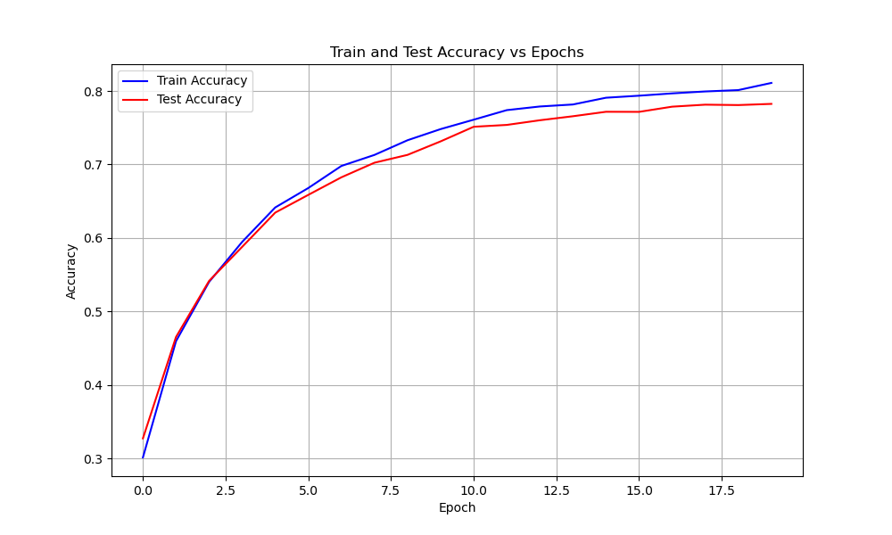
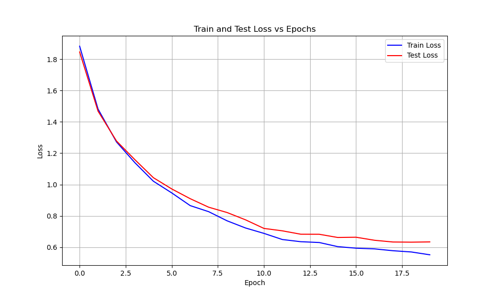
| Train | 0.8 | 0.59 | ||
| Test | 0.79 | 0.61 |