Phase 1

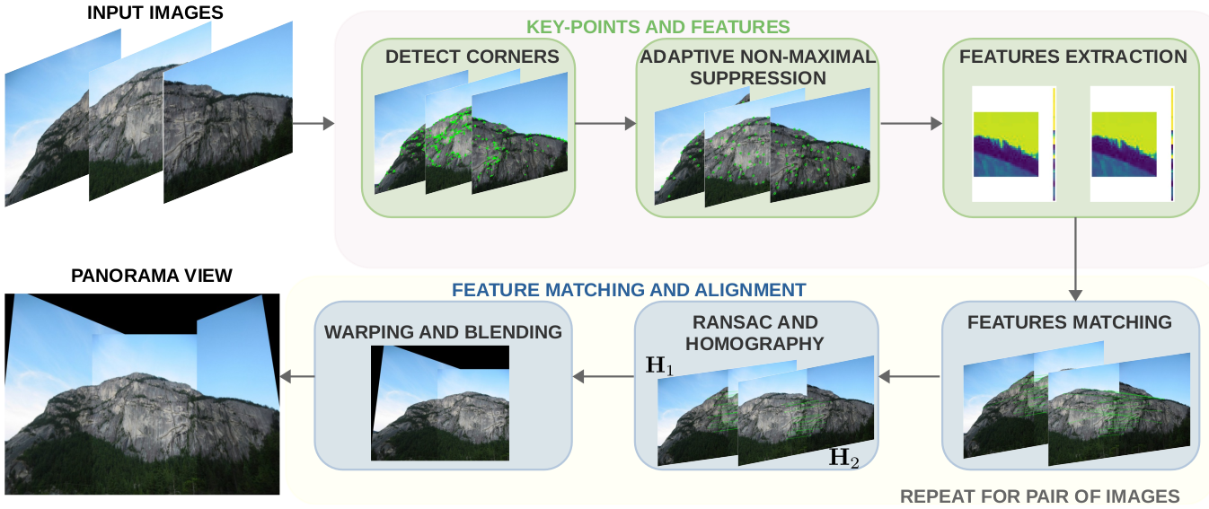
This section presents the implementation of panorama stitching considering the traditional formulation.The traditional approach involves the following steps: detecting key-points in images, extracting feature descriptors, and using Random Sample Concensus (RANSAC) to robustly estimate the homography matrix between images.

Corner Detection

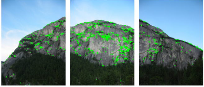
A corner in an image is a region where the gradient shows significant changes in multiple directions. The Harris Detector, a popular algorithm for corner detection, analyzes intensity variations in a pixel’s local neighborhood to identify such points.

Adaptive Non-Maximal Suppression

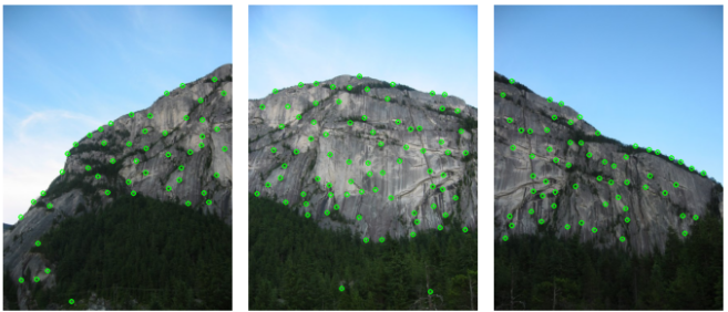
While the Harris detector successfully identifies corners in the image, these features are not uniformly distributed. The purpose of Adaptive Non-Maximal Suppression (ANMS) is to enhance the spatial distribution of key points. Specifically, it aims to select the Nbest most optimal corners by identifying those that are true local maxima.

Algorithm 1: Adaptive Non-Maximal Suppression
Data: Corner score Image C and the maximum of best corners
Nbest
Result: (xi , yi ) for i = 1 : Nbest
1 Initialized ri = ∞ for i = 1 : Nstrong ;
2 for i = [1 : Nstrong ] do
3 for j = [1 : Nstrong ] do
4 end
5 if C[yj ,xj ] > C[yi ,xi ] then
6 ED = (xj − xi )2 + (yj − yi )2 ;
7 end
8 if ED < ri then
9 ri = ED;
10 end
11 end
12 Sort ri in descending order and pick top Nbest points
    

Features Descriptor

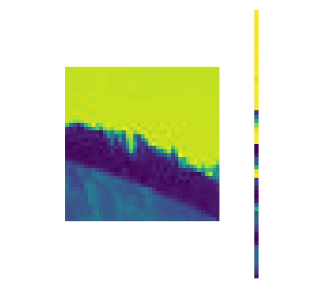
The next step is to generate descriptors that facilitate comparisons between these key points. Each key point is represented by a feature vector or descriptor, derived from a patch centered on the key point that captures its distinguishing features. Various methods can be used to generate feature descriptors, including Gaussian functions, gradient orientations, or texture-based approaches. In this work, we adopted a straightforward method by applying a Gaussian function to the patch and subsequently sub-sampling the resulting blurred output.

Features Matching

Now, the task is to identify the feature vector correspondences between the two images. To achieve this, for a given point in Image 1, we calculate the differences with all points in Image 2 and compute the squared Euclidean norm for each. Using this metric, we determine the ratio between the best match (lowest distance) and the second-best match (second lowest distance). If this ratio is below a predefined threshold, the match is retained; otherwise, it is discarded. We repeat this process for every feature point in Image 1.

Random Sample Consensus (RANSAC) for outlier rejection

In the previous section, we demonstrated the ability to match feature vectors between images. However, the results above reveal that we are identifying not only correct correspondences but also incorrect ones. To mitigate these matches, this work employs RANSAC method to compute the homography using only the accurate matches between images.

Algorithm 2: RANSAC
Data: Four feature matches from images P and P'
Result: Homography matrix H between pair of images
1 for i = [1 : Nmax ] do
2   P ← Four random features from image 1
3   P' ← Four random features from image 2
4   H ← (P1, P1') Compute homography
5   p' − Hp < τ Compute inliers
6   if inlier > 90% then
7       break;
8   end
9 end
10 Keep the largest set of inliers
11 Re-compute least-squares Ĥ
    

Image Stitching

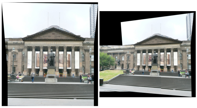
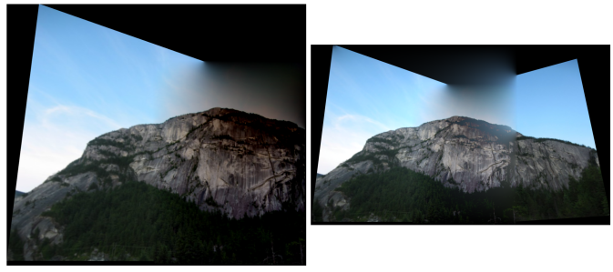
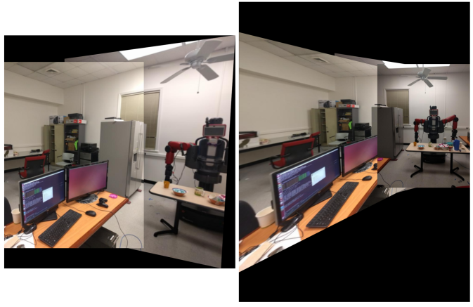
Once the homography matrix between the pair of images is obtained, it becomes possible to combine multiple views into a single image, resulting in a seamless panoramic view. However, in this technique, it is quite important to blend the common region between images without affecting the regions that are not common.

Poisson Blending: This technique is used to seamlessly blend one image into another when stitching multiple images. Poisson blending achieves this by transferring gradient information from the source image to the destination image while maintaining the overall smoothness of the stitched result. This approach is based on solving a Poisson equation for the image to ensure that the gradients from the second image are maintained while minimizing discontinuities at the boundary of the stitch.

Alpha Blending: This technique combines multiple images using the value alpha, which represents the transparency of each image. By enabling smooth transitions between the foreground and background, it is particularly well-suited for tasks such as image compositing.

Phase 2

This section presents the implementation of panorama stitching considering the deep learning network approaches. The deep learning approach can be performed in two different ways:

• Supervised Learning
• Unsupervised Learning

Dataset Generation

To train both supervised and unsupervised approaches for estimating homography between pairs of images, we need datasets comprising pairs with known homographies. The procedure of obtaining these datasets is generally challenging, as determining the homography requires knowledge of the transformations between image pairs. Consequently, synthetic pairs of images are generated to train the networks, using a small subset of images from the MSCOCO dataset, which encompasses a diverse array of objects in natural scenes. The steps to generate the images are as follows: Before generating image pairs, all the pairs should be of the same size and the first step is to resize the images to a standard dimension. In our implementation, we resize the images to 320x320.

• We then apply a random crop on the images in feature-rich regions using corner detection method. This is our original patch PA having corners CA.
• On this patch PA we apply random transformation HAB to get a perturbed patch with corners CB.
• We calculate the inverse homography HA that maps from the perturbed patch to PA and call this the patch PB that has the same coordinates in the transformed image as that of PA in the original image.

The dataset comprises 5000 images, from which 30 patches are generated for each image using the aforementioned procedures, resulting in a total of 150,000 images.

Supervised Approach

A supervised learning approach is a type of machine learning in which a model is trained on labeled data. This means that the algorithm learns from a dataset that already contains input-output pairs, where each input is associated with a correct output. In our implementation, the input of the model is the pair a pair of gray-scale image patches, and the ground truth labels are the homography between them. The objective of this optimization problem is to minimize the error between the estimated output of the neural network and the ground-truth homography. In this work we use the structure presented in HomographyNet.

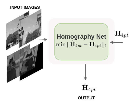
The patch size for each image is 128x128, and the patches PA and PB are normalized and stacked on top of each other to obtain a single input.

HomographyNet: We use the HomographyNet, a deep CNN having 8 convolutional layers and 2 fully connected layers. Each layer has 3x3 convolutional blocks with BatchNorm and ReLUs. The network takes as input a two-channel gray-scale image i.e the image stack PA and PB sized 128x128x2. We use 8 convolutional layers with a max pooling layer (2x2, stride 2) after every two convolutions. The 8 convolutional layers have the following number of filters per layer: 64, 64, 64, 64, 128, 128, 128, 128. The convolutional layers are followed by two fully connected layers. The first fully connected layer has 1024 units. Dropout with a probability of 0.5 is applied after the final convolutional layer and the first fully-connected layer. The output of the network directly produces 8 real-valued numbers which are the predictions of the difference of perturbation from CA to CB.

Hyperparameters: The hyperparameters used for the model are as follows:

• optimizer: SGD
• learning rate: 0.006
• loss metric: L1 norm
• epochs: 100
• batch size: 64

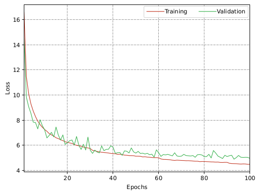
Experiments and Results: The model is trained on the dataset of size 150,000 image pairs for 100 epochs for about 8.0 hours on a single NVIDIA RTX GPU. Each image is resized to 320x320 dimensions and subsequently converted to gray-scale.

Unsupervised Approach

The unsupervised learning approach is a type of machine learning in which the model is trained using data that are not labeled, meaning that the input data do not have ground truth for comparison. In unsupervised learning, the goal is for the model to find patterns, relationships, or structures in the data without the need for explicit supervision.

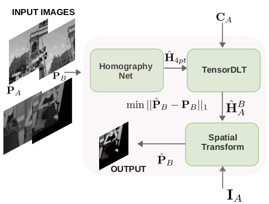
HomographyNet: The model pipeline is an extension of the previous model, where the same HomographyNet model is used and two more blocks are added, namely the TensorDLT and Spatial transformer blocks. The HomographyNet model works the same way in the forward iteration of the model giving the same H4pt output.

• The TensorDLT layer takes this output and the corners CA and calculates the estimated homography H̃BA.
• The spatial transformer takes the original image IA and warps it using estimated homography to give an estimated image I˜B .
• Using the coordinates CA we extract the estimated patch P̃B from the estimated image I˜B .
• The patches PB and P̃B are compared using L1 loss function and the weights of the model are updated to reduce this loss.

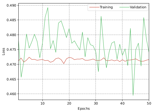
Hyperparameters: The hyperparameters used for the model are as follows:

• optimizer: SGD
• learning rate: 0.0001
• loss metric: L1 norm
• epochs: 50

Experiments and Results: The model is trained on the dataset of size 150,000 image pairs for 50 epochs for about 12 hours on an NVIDIA A30 GPU. All images are resized to 320x320 and converted to grayscale as done for the supervised training. The inputs are provided to the model and the H4pt values are obtained which are given to the tesnorDLT layer along with CA to obtain the estimated homography matrix. We use kornia transform to warp the image IA to obtain the estimated image I˜B . Applying the coordinates CA to I˜B gives us the estimate patch P̃B . The loss L1 is calculated for PB and P̃B and the model weights are updated based on the loss value.