Problem Statement

Trajectory following with PID and LQR Controllers.
Integrate the trajectory generator and controller to simulate the quadrotor flying in the space tracking a trajectory. Combine with PD controller. In addition you implement a LQR controller for the quadrotor, combine with trajectory generation system designed at previous step, see if the results are better compared to using PID/PD controller.

LQR Implementation

The state vector of the quadrotor is taken as:

$$ X = \left[\begin{array}{c} x \\ y \\ z \\ \dot{x} \\ \dot{y} \\ \dot{z} \\ \phi \\ \theta \\ \psi \\ p \\ q \\ r \end{array}\right] $$

where p is the angular velocity around x, q is the angular velocity around y and r is the angular velocity around z.

The rate of change of state vector is then calculated as:

$$ X = \left[\begin{array}{c} \dot{x} \\ \dot{y} \\ \dot{z} \\ \ddot{x} \\ \ddot{y} \\ \ddot{z} \\ \dot{\phi} \\ \dot{\theta} \\ \dot{\psi} \\ \dot{p} \\ \dot{q} \\ \dot{r} \end{array}\right] $$

where $\dot{p}$, $\dot{q}$ and $\dot{r}$ are the angular accelerations around x,y and z.

Now we can write the state space equation as:

$$ \dot{X} = f(X,U) $$

We can use Taylor’s approximation to Linenarize the above equation to get:

$$ \dot{X} = AX + BU $$

where A is the Jacobian obtained by partially differentiating f(X,U) with X and B is the Jacobian obtained by partially differentiating f(X,U) with U.

The Q and R matrices have been calculated by trial and error method where

$$ Q = diag([20,20,20,1,1,1,0.01,0.01,0.01,0.01,0.01,0.01]) $$

$$ R = diag([0.001,0.1,0.1,0.1]) $$

which penalizes the cost function more for position and velocity errors in the state and penalizes the control of x,y and z moments.

Results

1. Circle

The results for the circular trajectory comparing both PD control and LQR control are given below:

Circular Trajectory

Position Tracking

Velocity Tracking

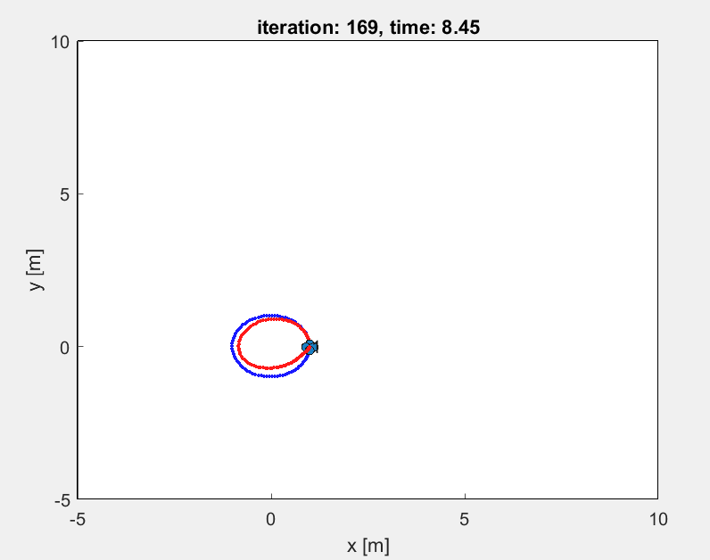
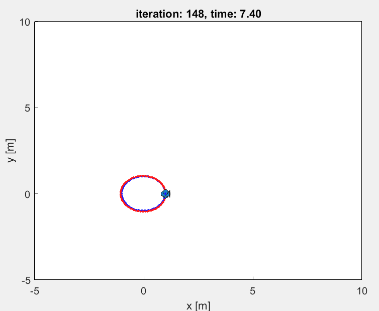
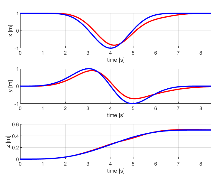
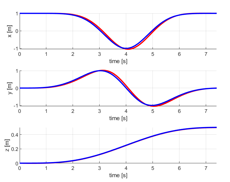
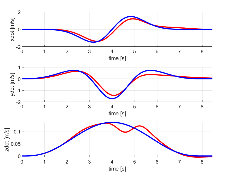
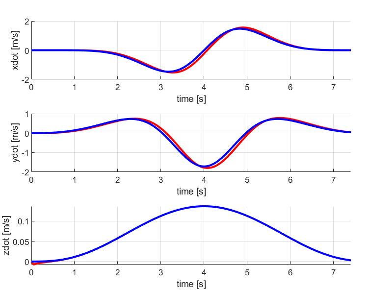
As seen from the above comparison, the LQR tracks the circular trajectory in a better way than the PD control method. The desired and current position and velocity curves are much closer in LQR graphs than in PD controller graph.

2. Diamond

The results for the diamond trajectory comparing both PD control and LQR control are given below:

Diamond Trajectory

Position Tracking

Velocity Tracking

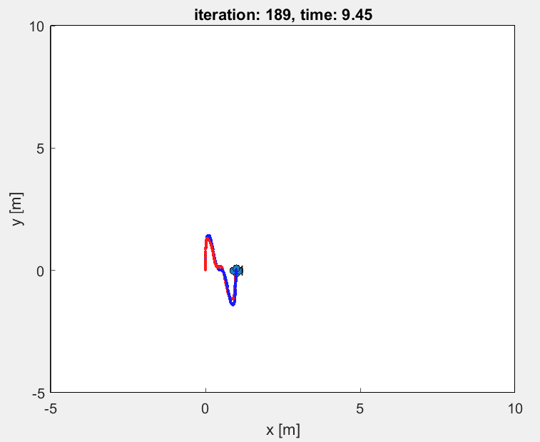
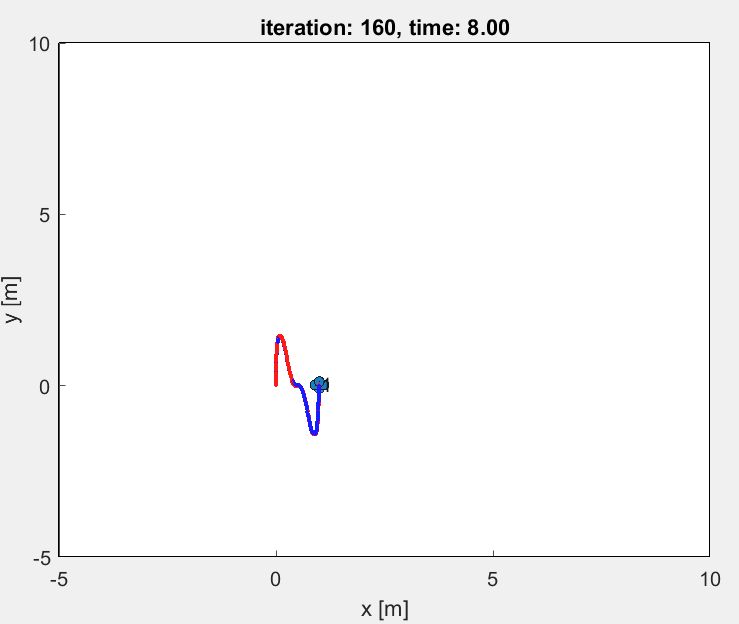
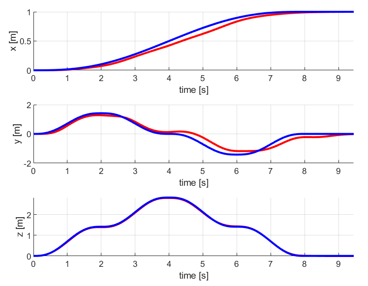
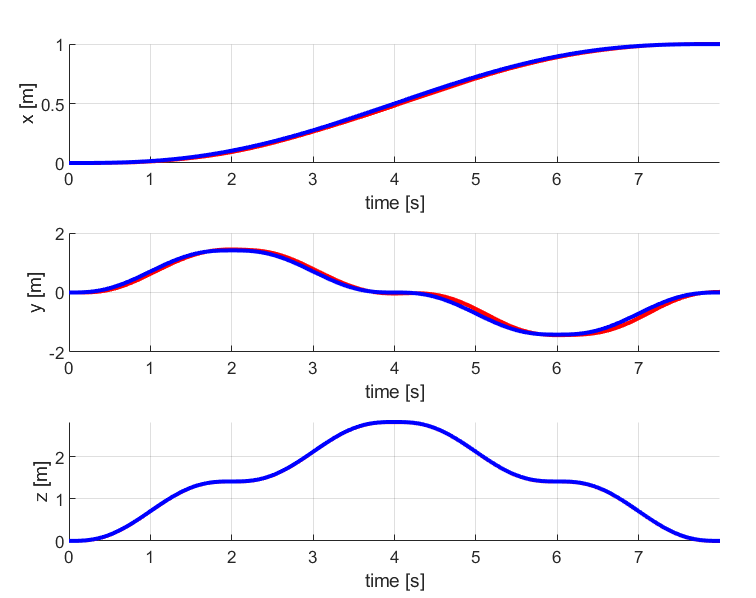
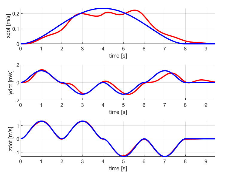
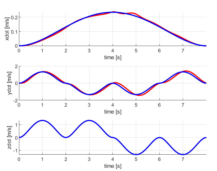
Similar to the circular trajectory case, the LQR tracks the diamond trajectory in a better way than the PD control method.
The desired and current position and velocity curves are much closer in LQR graphs than in PD controller graph.
From the above comparisons, we can see that LQR minimizes the cost function based on the Q and R values and provides an optimal control solution that tracks the desired trajectory closely by taking advantage of the full state feedback control.
However, LQR has a few drawbacks too.
LQR requires solving the Riccati Equation which is mathematically complex and comaputationally expensive to solve especially for high dimensional systems.
LQR assumes a perfectly known system model. If the system model is inaccurate or subject to significant uncertainties, the performance of the LQR controller may degrade or become suboptimal.